Radiative Cooling Strategies for Habitat Sustainability

Operational Intelligence Through Capacity Monitoring and Design Patterns for Scalable Thermal Infrastructure

Introduction

Habitable environments generate thermal energy through solar heating, electrical equipment and biological activity. Without adequate heat rejection, temperatures rise beyond acceptable limits to maintain safe living and working conditions. Radiative cooling provides an inexpensive solution for removing this thermal energy by rejecting heat into space.

Many radiative solutions minimize electrical consumption, but provide limited insight into thermal load characteristics. Supplementary monitoring systems can fill this gap by offering real-time performance metrics but are constrained—historical data retention is limited and dedicated monitoring controllers add complexity and cost. Simple metrics that can be read at a glance become essential for practical operation.

This architecture presents a single physical configuration that can support multiple heat rejection strategies, allowing operators to select the appropriate balance of power consumption, control precision, and diagnostic capability for specific applications. It accommodates three distinct control regimes within one standardized layout, tunable through molar quantity adjustment, rather than physical reconfiguration.

System Architecture

This specification defines a standard cooling unit with established operating parameters and performance characteristics. Operators can deploy and replicate this build across installations in order to assess capacity utilization and make informed scaling decisions.

Operating Parameters

Room Pressure: Max atmospheric pressure (101.325 kPa)

Atmospheric Composition: For typical habitable sectors:

• 20% O₂ (oxygen for respiration)

• 77% N₂ (inert atmospheric buffer)

• 2% CO₂ (sufficient for plant growth)

• <1% Others (contaminant tolerance + composition margin)

Room Temperature: Minimum: 20°C (293.15K) with a setpoint range of 20-30°C

Performance Specification

Cooling Rate: 5K temperature reduction in under 10 minutes¹ ²

Sector Coverage: Maximum 159 GU volume

Test Condition: No baseline thermal load

Energy Removal Capacity: Minimum 4373 J/tick

Build Specification

The standard configuration supports two models: cold loop passive (CLP) systems use a mechanical valve with no electrical power requirements and cold loop active (CLA) systems use a digital valve and pump for precise capacity modulation. Both share identical pipe layouts and radiator configurations.

Combined system diagram showing cold loop passive (left) and cold loop active (right) configurations

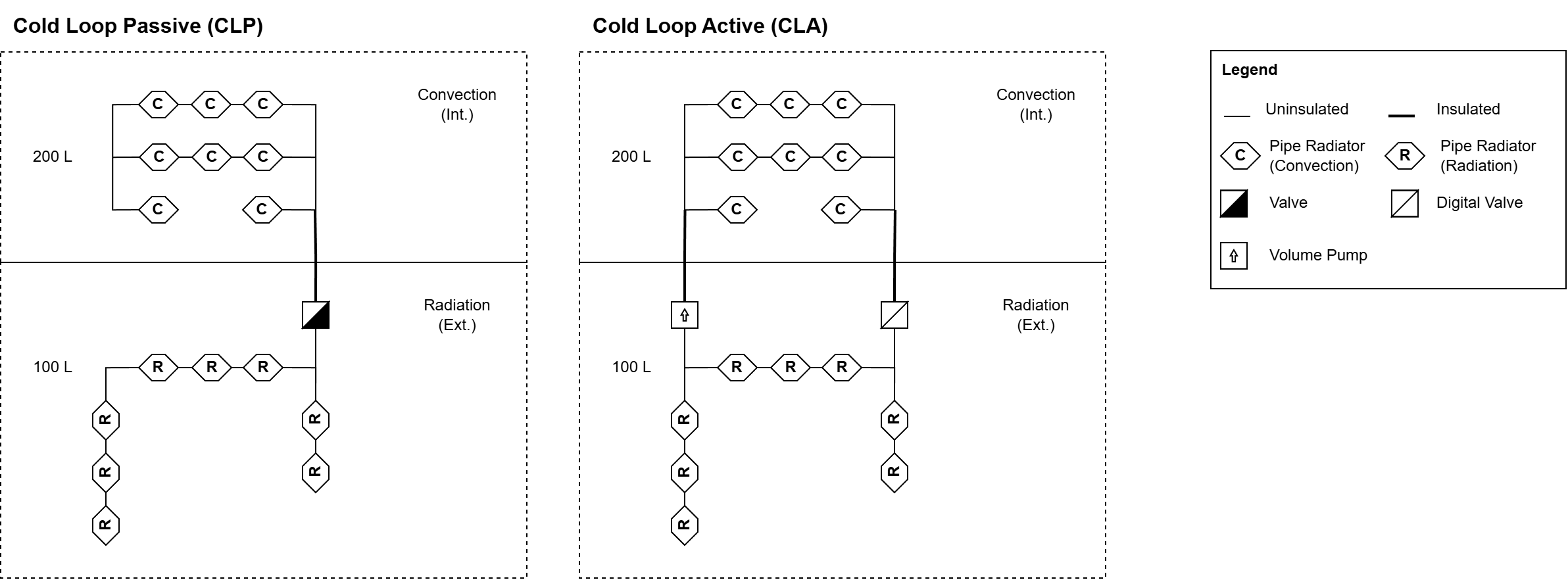
Pipe Configuration: 300 L total pipe volume

• Convection segment: 200 L (interior)

• Radiation segment: 100 L (exterior, vacuum exposed)

Radiators: 16 pipe radiators total

• Convection segment: 8 convection pipe radiators

• Radiation segment: 8 pipe radiators

Working Fluid: Carbon dioxide (13.011 mol)³

System Models

The system architecture describes two separate build models: CLP and CLA. Using the same pipe configuration, each solution offers a different balance of power consumption, temperature control precision and monitoring telemetry.

CLP (Cold Loop Passive)

CLP models use mechanical valves and require no electric power. Cooling capacity is directly proportional to gas quantity, with no thermostatic control capability.

Application: Guaranteed thermal loads that would not be impacted by power failures, such as solar heating effects and averaged biological heat loads.

Limitations: No active temperature control or transient response capability. System reaches thermal equilibrium based on fixed cooling capacity versus heat input.

CLA (Cold Loop Active)

CLA models use a gas sensor, digital valve, pump, IC, and PID to regulate cooling capacity. A single controller supports two runtime modes selectable via manual switch, allowing operators to choose between power efficiency and operational visibility based on current needs.

The ability to switch modes on a per-system basis allows for targeted capacity assessment without running all cooling systems in high-power mode continuously.

Thermal Pulse Mode (75 W average)

Thermal pulse mode cycles between active cooling and standby states based on thermostatic thresholds. When monitored temperature exceeds the upper threshold the valve opens, circulating gas through the entire radiator loop. Once temperatures drop below the lower threshold, the pump activates, evacuating the radiation segment, and the system returns to standby.

Application: Power efficient cooling for well-characterized thermal loads where temperatures vary within acceptable ranges. Suitable for routine operations when capacity margins are known and precise control is unnecessary.

Limitations: No capacity monitoring. System either maintains temperature within range or fails to do so with no advance warning.

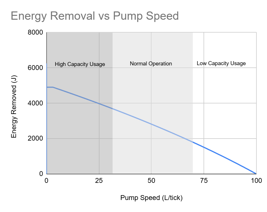
Thermal Tracking Mode (675-875 W)

Thermal tracking mode maintains precise temperature control around a setpoint by using pump speed to actively regulate gas flow through the radiation pipe segment. The pump operates continuously, with speed inversely proportional to cooling demand — lower speeds provide maximum cooling capacity by increasing gas pressure within the radiation segment.

Telemetry: Pump speed serves as a diagnostic metric for capacity utilization. Low pump speeds under normal conditions indicate the system approaching capacity limits, providing early warning to scale out cooling infrastructure before thermal control fails.

Lower pump speeds correspond to higher energy removal, enabling real-time capacity assessment through speed monitoring alone.

Applications:

• Initial deployment for thermal load characterization

• Troubleshooting problem areas where heat dissipation needs to be quantified

• Critical systems that require precise temperature control

• Variable thermal loads where capacity monitoring provides usage data

Limitations: Highest power consumption. Unnecessary for simple and stable thermal loads.

Multi-System Deployments

Large sectors with shared atmospheres may benefit from layered cooling strategies:

Sector Thermal Tracking System: A single controller manages multiple CLAs and operates in thermal tracking mode to monitor aggregate sector temperature, provide baseline cooling capacity, and offer sector-wide thermal stability. Sector thermal systems support up to 6 thermal tracking units per controller on a 5 kW cable or small transformer network.

Dedicated Thermal Pulse Systems: Independent systems handle localized heat sources, and monitor its own specific 1 GU volume near equipment clusters. These operate autonomously based on local thermostats without coordination.

Cold Loop Passive Baseline: Provides zero-power cooling for solar and biological loads and ensures minimum thermal control during power failures.

Power and Network Design

Cooling systems deploy in two distinct configurations based on operational context: dedicated thermal systems for localized equipment cooling, and sector thermal systems for ambient thermal management. The deployment strategy determines network architecture, power requirements and control topology.

DTS (Dedicated Thermal System): Deploy as child networks of high-heat generating equipment, integrating cooling power budget into the equipment’s usage overhead. When equipment loses power and stops generating heat, the cooling system automatically shuts down, eliminating wasted energy.

STS (Sector Thermal System): Deploy as independent sector infrastructure, managing distributed ambient loads from lighting, doors, and low overhead equipment that do not warrant dedicated cooling hardware. STS operate continuously regardless of individual equipment states.

DTS (Dedicated Thermal System)

DTS integrate into equipment power hierarchies as child networks. The cooling system transformer connects downstream of the equipment’s system transformer, creating an explicit dependency: equipment power loss cascades to cooling system shutdown.

Isolated system network topology as a child network of parent system (see Network Topology Reference for diagram notation)

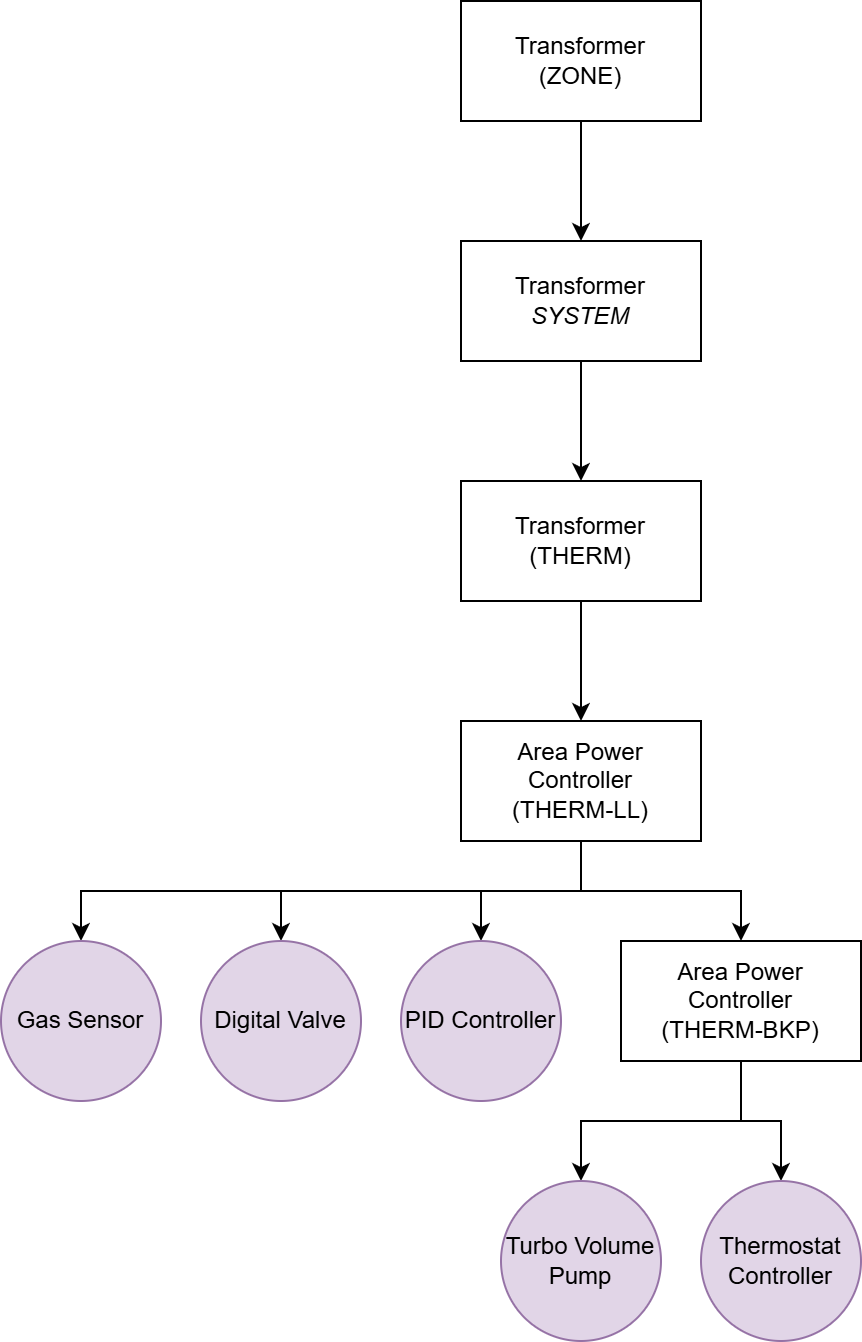
Thermal Pulse Mode (75 W): The THERM-LL APC with large battery buffers intermittent pump operation characteristic of thermal pulse cycling. Without load leveling, thermal pulse systems create brief power demand spikes at the end of cooling cycles. The large battery smooths these transients, presenting steady average power draw to the upstream transformer.

Thermal Tracking Mode (875 W): Thermal tracking systems operate the pump continuously at variable speeds, creating steady power demand without transient spikes. Adding a battery at the load-leveling junction is unnecessary and can be omitted—as the device acts a passthrough from the THERM transformer.

Graceful Degradation: The backup controller (THERM-BKP) uses a small battery to ensure controlled shutdown during power failures. This ensures that the radiation pipe is fully evacuated to prevent damage to infrastructure.

STS (Sector Thermal System)

STS deploy as sector infrastructure, managing ambient thermal loads independent of specific equipment states. The cooling system connects directly to the zone transformer without intermediate system-level transformers, indicating it serves general sector operations rather than dedicated equipment.

STS system network topology as general sector infrastructure

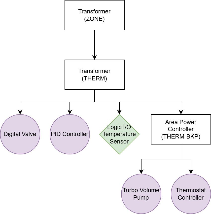
Sensor Aggregation: STS use a Batch Reader (Logic I/O) to compute the average temperature from gas sensors in the Life Support Network. This eliminates redundant sensors and enables coordinated response across all units in the batch.

Scaling Limits: STS support up to 6 load-matching units per controller on 5 kW cable or small transformer junction. Beyond 6 units, deploy additional STS or upgrade power infrastructure to support additional load.

Installation Requirements: Each unit in the STS requires two connections to shared networks:

• Valve power/data to THERM Transformer

• Pump power to THERM-BKP Area power controller

• Pump data to THERM Transformer

Links to Implementation

For operators ready to deploy the radiative cooling system within their own base, the following implementation guide walks through the full construction process—complete with layout considerations, materials, and programmable logic:

• Life Support III: Radiative Cooling - Construction guide for deploying a Dedicated Thermal System (DTS) in a starter greenhouse environment. Covers physical installation, power network configuration, gas pressurization, and how to interpret PID signals for operational capacity assessment.

Appendix

A1. Thermal Transfer Calculations

Note: The follow thermal transfer formulas were reverse-engineered through empirical testing by @GKuba. Documentation available in the Stationeers Discord: https://discord.com/channels/276525882049429515/395912153795788803/1393151312983621703

Convective Heat Transfer

Convection occurs between gas in pipes and gas in adjacent rooms/volumes:

\(E_c = min(50 \times N_\text{room} \times N_\text{pipe} \times k_c \times (T_\text{room} - T_\text{pipe}), E_h)\)

Where:

• E_c = convective heat transfer (J)

• N_room = pressure normalization factor for room gas

• N_pipe = pressure normalization factor for pipe gas

• k_c = thermal convection coefficient (found in Stationpedia)

• T_room = room gas temperature (K)

• T_pipe = pipe gas temperature (K)

• E_h = thermal equilibration limit

Thermal Equilibration Limit

\(E_h = \frac{\dot{C}_\text{room} \times \dot{C}_\text{pipe}}{\dot{C}_\text{room} + \dot{C}_\text{pipe}} \times (T_\text{room} - T_\text{pipe})\)

Where:

• Ċ_room = thermal mass flux for room gas, characterized by the product of molar quantity and specific heat capacity (n × c)

• Ċ_pipe = thermal mass flux for pipe gas

Pressure Normalization

\(N_n = min(\frac{P_n}{P_\text{atm}}, 1)\)

Where:

• P_n = pressure in the volume (kPa)

• P_atm = standard atmospheric pressure (101.325 kPa)

Pressure normalization caps at 1.0, meaning pressures above atmospheric do not increase heat transfer beyond normalized rate.

Radiative Heat Transfer

The following formulas apply specifically to vacuum environments:

\(E_r = min(N_\text{pipe} \times k_r \times U(T_\text{pipe}), \frac{E_k}{2})\)

Where:

• E_r = radiative heat transfer (J)

• N_pipe = pressure normalization factor

• k_r = thermal radiation coefficient (found in Stationpedia)

• U(T_pipe) = entropy function of pipe gas temperature

• E_k = internal energy of gas in the pipe (n × c × T_pipe)

Entropy Function

\(U(T) = a \times (T-50)^3 + b \times (T-50)^2 + c \times (T-50) + d\)

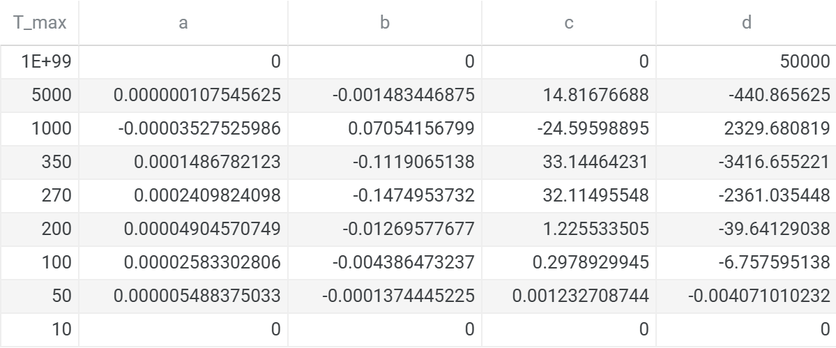
Where T is the pipe temperature in Kelvin, and coefficients a, b, c, d vary by temperature range (see table below).

Energy Curve Coefficients

A2. Window Thermal Characteristics

Solar Heating Through Windows

Windows admit solar radiation into habitable environments, creating continuous thermal loads that must be managed through cooling systems. The magnitude of solar heating depends on window area, solar intensity, and environmental conditions.

Heat Input per Window Panel

Empirical testing has established approximate heat input values for standard window configurations on the moon. A single window panel admits approximately 77 W of thermal energy under normal daytime solar conditions when oriented to receive direct solar exposure.

Window Orientation: North-South facing windows (perpendicular to solar path) do not appear to contribute measurable heat input. Only windows with direct solar exposure (East-West facing, or angled to intercept sunlight) generate thermal loads. This allows strategic window placement for visibility without proportional cooling requirements.

This value accounts for the Moon’s 2× solar irradiance multiplier compared to Mars’ baseline measurements. Community analysis of Martian window performance adjusted for lunar conditions, provides the comparison for these estimates.

Source: https://www.reddit.com/r/Stationeers/comments/14p7opq/on_mars_how_much_heat_does_the_sun_add_to_a/

Solar Storm Conditions

Solar storms increase energy output from solar panels by 4× normal values. Window heat admission scales proportionally, creating approximately 308 W thermal input per window panel during solar storm conditions.

Solar storms typically last around 5 minutes (half a day cycle), creating transient thermal spikes that cooling systems must accommodate.

CLP Sizing Guidelines

A CLP unit’s capacity can be characterized through window count. Under normal conditions, each window panel utilizes a daytime system load of about 0.875%, averaging at around 0.4375% over a lunar day. That means, at full capacity, a single passive regulated unit could theoretically support up to 228 windows worth of solar heating. This estimation assumes:

• Windows concentrated in areas served by passive cooling

• Adequate atmospheric mixing without creating cold spots in non-windowed areas

• Passive system sized with standard 13.011 mol CO₂ charge

• No thermal spikes caused by transient solar storm events

Downsizing Capacity

Operators can reduce heat removal capacity of a passive system by proportionally reducing the mole count. For example, a 4 GU greenhouse with 8 windows utilizes an average of 3.5% heat removal capacity over a lunar day (8 windows ×0.4375% per window). To calculate the moles to pressurize the system, multiply the standard charge by the average utilization:

\(13.011 \times 0.035 = 0.455 \text{ mol}\)

A3. Thermal Simulation Spreadsheet

The system architecture was designed to determine the largest cooling unit supported by a single 100 L turbo pump with full evacuation capability. This appendix documents the simulation methodology used to establish the 300 L configuration with 13.011 mol CO₂ charge.

Thermal Pulse Simulation (Baseline)

Room Input Parameters

Average Specific Heat: Calculate based on target atmospheric composition. For lunar habitats with breathable atmosphere (77% N₂, 20% O₂, 2% CO₂), use a weighted average of component specific heats.

Pressure: Maximum operating pressure, capped at atmospheric (101.325 kPa). This establishes worst-case thermal mass for equilibration calculations.

Volume: Total habitable volume in liters (GU count × 8000L). This determines the thermal mass for equilibration between room and pipe gas.

Minimum Room Temperature: Lowest acceptable operating temperature (293.15 K/ 20°C). Colder gas temperatures reduce heat removal capacity, establishing a conservative design point.

Pipe Input Parameters

Pipe Specific Heat: 28.2 J/(K•mol) (Carbon dioxide)

Radiation Segment:

• Volume (V_c): 100L (fixed by pump evacuation constraint)

• Radiation coefficient (k_r): 27.68

  • Calculation: 8 radiators (3.46 per radiator) / 80 L pipe + 20L junction pipe

  • 8 radiators = maximum supported by 100 L evacuation volume

Convection Segment (initial guess):

• Volume: Start with V_c = V_r = 100 L

• Convection coefficient (k_c): 6.34

  • 6 radiators (1.05 per radiator) / 60 L pipe (0.03 at 0.005 per pipe) + 20 L junction (0.01 at 0.005 per pipe) + 20 L wall penetration pipe

  • Note: Radiators cannot contact walls (reduces effectiveness)

Molar Quantity (initial guess):

Calculate pipe moles at minimum room temperature and atmospheric pressure using ideal gas law:

\(\begin{align} n_\text{total} &= \frac{PV}{RT} \\\\ &= \frac{101.325 \times 200}{8.314 \times 293.15} \end{align}\)

This establishes baseline even though pipe temperature will be colder in operation.

Simulation Structure

Initial Conditions (time=0):

• Room Temperature: Select starting temperature

• Pipe Temperature: Same as room temperature (valve closed, no gas in radiation segment)

• Room Pressure: Can model as constant pressure (variable moles) or constant moles (variable pressure). Design uses constant atmospheric pressure with variable mole count.

• ΔT: Room Temperature - Pipe Temperature = 0 initially

• Convection, Radiation Pressure (P_c, P_r): Calculate from ideal gas law using pipe temperature, segment volumes and total molar count (equal initially with no flow)

• Load: User-defined thermal input (J)

• Convection, Radiation Energy (E_c, E_r) : Calculate using formulas from Appendix A

Time Step Iteration (t > 0): Duration 1200 ticks (10 minutes) for system architecture

For each tick:

1. Room Temperature:

   \(T_\text{room}(t) = \frac{m_\text{room} \times c_\text{room} \times T_\text{room}(t-1) + E_\text{load} - E_c}{m_\text{room} \times c_\text{room}}\)

2. Pipe Temperature:

   \(T_\text{pipe}(t) = \frac{m_\text{pipe} \times c_\text{pipe} \times T_\text{pipe}(t-1) + E_c - E_r}{m_\text{pipe} \times c_\text{pipe}}\)

Iterative Refinement:

1. Run simulation until pipe reaches minimum room temperature

2. Capture energy removed and gas pipe temperature at this point

3. Recompute optimal molar quantity for these conditions

4. Determine maximum convection pipe volume where E_c ≥ E_h at atmospheric pressure, minimum pipe temperature and no gas flow

5. Adjust k_c to the new pipe volume

6. Repeat until the system converges on a reasonable maximum capacity

Thermal Matching Simulation (Flow Modulation)

Thermal matching mode uses pump speed to modulate gas distribution between convection and radiation segments. Lower pump speeds increase gas pressure in the radiation segment, providing higher cooling capacity.

Flow Rate Modulation

Pump Speed (p): p = V_r × x

Where x represents the control output (0 to 1)

Maximum Molar Flow Rate:

\(\dot{n}_\text{max} = n_\text{total} \times \frac{V_r}{V_r+V_c}\)

Radiation Segment Molar Quantity (n_r):

\(n_r = \begin{cases} x \times \dot{n}_\text{max} \times \frac{V_r - p}{p}, & p > 0 \\ \dot{n}_\text{max}, & p = 0 \end{cases}\)

Convection Segment Molar Quantity (n_c):

\(n_c = V_c \times \left(x \times \dot{n}_\text{max} \times \frac{V_c+V_r}{V_cV_r} + \frac{n_r}{V_r}\right)\)

Segment Pressures: Calculate P_c and P_r from ideal gas law using n_c, n_r, respective volume and pipe temperature.

A4. Glossary

This glossary defines terminology specific to the radiative cooling architecture documented in this article. For broader Stationeering Systems terminology, refer to the Terminology Reference.

CLA (Cold Loop Active) — “claw” Powered cooling system using digital valves and pump equipment for thermal capacity modulation. CLAs support two operating modes (TPM and TTM) selectable via manual control input.

CLP (Cold Loop Passive) — “clap” Unpowered cooling system using mechanical valves. Cooling capacity is proportional to gas quantity, with no active temperature control capability.

Capacity Utilization — Fraction of maximum cooling capacity currently in use. In thermal tracking mode, indicated by pump speed: lower speeds correspond to higher capacity utilization (more cooling demand). Operators monitor capacity utilization to determine when additional cooling units are required.

Convection Segment — Interior pipe network where gas absorbs thermal energy from adjacent atmosphere.

DTS (Dedicated Thermal System) — Cooling system deployed as child network of specific equipment. The DTS transformer connects downstream of the equipment’s system transformer, creating explicit dependency. When parent equipment loses power and stops generating heat, the DTS automatically shuts down.

Radiation Segment — Exterior vacuum-exposed pipe network where gas rejects thermal energy to space through passive radiation.

STS (Sector Thermal System) — Cooling system deployed as independent sector infrastructure for ambient thermal management. Multiple cooling units controlled by centralized sensor aggregation with shared control logic. Handles distributed loads from lighting, doors, and small equipment not warranting dedicated cooling.

Thermal Pulse Mode — Operating mode for CLA systems. Cycles between active cooling and standby states based on temperature thresholds. Valve opens and pump activates when temperature exceeds upper threshold, returns to standby when temperature drops below lower threshold.

Thermal Tracking Mode — Operating mode for CLA systems. Uses continuous pump speed modulation to match cooling capacity to current thermal load. Pump speed inversely correlates with cooling demand; lower speeds provide higher cooling output.

A5. References

• Stationeers Official. Atmospheric System Update https://store.steampowered.com/news/app/544550/view/530986717166960683

• Stationeers Discord. @GKuba - Thermal Transfer Formulas https://discord.com/channels/276525882049429515/395912153795788803/1393151312983621703

• Stationeers Discord. @GKuba - CFHE Formulas
  https://discord.com/channels/276525882049429515/395912153795788803/1398761976477384755

• Reddit. Window Solar Heating Analysis (Mars) https://www.reddit.com/r/Stationeers/comments/14p7opq/on_mars_how_much_heat_does_the_sun_add_to_a/

• Reddit. Heat Generation Sources Discussion https://www.reddit.com/r/Stationeers/comments/15u2nha/what_generates_heat_in_a_room/

• Steam Community. Radiator Mechanics Discussion https://steamcommunity.com/app/544550/discussions/0/4691154153116885645/

• YouTube. Stationeers: PID Controller Chip

  https://www.youtube.com/watch?v=xxMOSAprx6M

---

Content developed in collaboration with Anthropic’s Claude, used for drafting, editing, and technical validation.

1. The 10-minute cooling specification represents a full nighttime cycle, establishing the system’s ability to recover from thermal transients within relevant timeframes.

2. The 5K/10-minute specification measures maximum cooling capacity under idealized conditions (no ongoing heat input). Within the environment, thermal loads from electrical equipment, solar heating and biological activity generate heat continuously. This system maintains equilibrium by matching heat removal to heat input rather than performing discrete cooldown cycles.

3. This molar quantity provides thermal mass for maximal heat throughput while maintaining atmospheric pressure at minimum pipe temperatures. This enables load-matching where cooling capacity responds to pump speed variations. Molar quantities above this standard provide diminishing returns —the system reaches pressure saturation where additional moles increase thermal equilibration capacity, but do not improve heat transfer rates proportionally.