
Microgrid Architecture for Resilient Power Systems
Hierarchical power distribution for graceful degradation and pre-emptive response
Introduction
Establishing network segmentation early provides protection against cable failures and simplifies troubleshooting as outlined in previous guides on power capacity planning and solar infrastructure design. Beyond initial segmentation, new challenges emerge: wiring complexity, cable overload, and sudden blackouts.
These problems are addressed through explicit load prioritization and measured capacity utilization. When power is constrained, the system determines which loads to maintain and which to shed based on defined priorities. Capacity monitoring tracks consumption against transformer limits, revealing when the grid nears exhaustion.
Source-Agnostic Design
This architecture treats power generation and power distribution as separate concerns. Stipulating that all power flows through a battery array, regardless of generation source, offers several advantages:
Decoupling generation from consumption: Generation sources charge batteries; distribution systems draw from batteries. Changes to generation infrastructure (adding solar panels, diversifying generation sources) require no modifications to the distribution topology.
Unified capacity planning: Battery charge represents available energy budget. Distribution systems allocate this budget across competing loads without regard to how the batteries were charged.
Consistent regulation behavior: Load management algorithms operate on battery state and discharge rates to provide stable control logic independent of generation variability (solar eclipses, fuel supply interruptions, wind fluctuations).
Hierarchical Organization
Power distribution uses three organizational levels to manage complexity at scale:
Region: Represents an allocation of distribution capacity, independent of generation source. A region supports up to 36 subnetworks, spread across 6 zones (one transformer assigned to each device pin). Region boundaries are determined by generation capacity limits, maximum subnetwork count, or practical management constraints—monitoring systems have location limits, and delivering systems like doors and lighting through a single region may become impractical or infeasible.
Zone: A capacity-limited subdivision within a region, supported by either medium or large transformers. Zones provide load guarantees with respect to cable management and support up to 6 subnetworks (one transformer assigned to each device pin).
Subnetwork: The smallest subdivision, representing equipment groups powered through a single zone connection point. Subnetworks can be reassigned between zones without major physical infrastructure changes, enabling dynamic reprioritization.
This hierarchy maps power topology to sectors, while maintaining electrical independence. A sector may contain multiple regions, but no region spans multiple sectors.
Design Objectives
Graceful degradation: When power capacity is insufficient, the system sheds non-critical loads in controlled priority order, allowing more critical networks to remain online for longer durations. Without this mechanism, inadequate power supply would force all network devices to go offline or sharply reduce available charge capacity.
Pre-emptive response metric: Capacity utilization monitoring reveals how closely actual consumption matches planned estimates. Operators use this metric to support expansion planning—adding generation sources, battery capacity, cable throughput, zones/regions before shortages occur. This complements initial capacity planning by validating assumptions against measured reality.
Architecture Overview
Power distribution follows a three-tiered structure that maps to how the control system manages allocation:
Region → Zone → Subnetwork
Regions represent the total distribution capacity from the battery array. Zones provide allocation granularity—the region control system allocates power budget to zones based on their priority and requested capacity, then each zone’s controller distributes its allocation among its subnetworks. Subnetworks represent the actual equipment consuming power.
This structure exists to manage control complexity. A flat system with 36 subnetworks directly connected to a region would require the regional controller to evaluate all 36 priority levels, capacity requests, and actual consumption values simultaneously. By introducing zones as an intermediate layer, the regional layer only evaluates 6 zones (manageable within controller processing constraints), and each controller independently manages up to 6 subnetworks.
The hierarchy is a control architecture, not an electrical necessity. Electrically, a region could directly power all subnetworks. The zone layer exists because the allocation algorithm benefits from breaking the problem into smaller, parallelizable decisions.
Network Flexibility
There are minimal restrictions on transformer selection, though practical considerations inform typical configurations.
Zone transformers: Medium (25 kW) or large (50 kW) transformers. With the 6-subnetwork limit per zone, maximum zone consumption is a little more than 30 kW (6 × 5 kW), making medium transformers the more common choice.
Subnetwork transformers: Typically small (5 kW) transformers. Small transformers expose their data network on the input side, allowing direct connection to zone network infrastructure. Medium and large transformers expose their data network on the output side (the distribution line), requiring an additional logic mirror to relay data back to the zone network. For subnetwork loads under 5 kW, small transformers avoid this additional complexity.
Redundancy Patterns
Expanding the base’s energy footprint allows for multiple strategies in how systems relate across regions based on criticality and failure tolerance requirements.
Independent Systems
Most systems exist independently within regions without cross-regional coordination or failover. Each region may have its own lighting network, thermal management, and monitoring infrastructure, or these systems may exist in only some regions based on operational needs. When these systems do exist in multiple regions, they share similar purposes, but operate in isolation—Region A-1’s lighting has no relationship to Region A-2’s lighting beyond nomenclature.
Independent systems accept complete downtime if their region fails. A power failure within the region disrupts power to those systems while adjacent regions continue normal operation without assuming additional responsibilities.
Dual-Region Interconnections
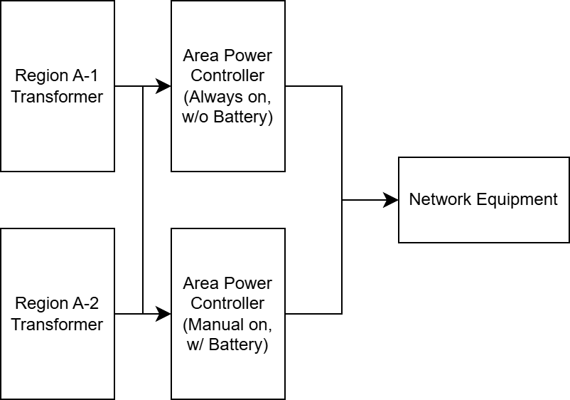
Equipment at regional boundaries connect to both regions simultaneously, drawing power from whichever region is available. Bypass doors and airlocks maintain this dual-feed configuration to prevent isolation scenarios where a single region failure might trap operators or block emergency egress.
Dual-region interconnections occur at sector boundaries (for doors between different sectors) and within sectors (doors between intra-sector regions). A passive battery backup provides tertiary protection so that if both regions fail, doors can still draw power from local battery storage to ensure access during compound failures.
This pattern differs from independent regional systems in active connectivity. A door connecting between Region A-1 and Region A-2 is not “Region A-1’s door” or “Region A-2’s door”—it simultaneously belongs to both regions.
N+1 Critical Systems
Survival-critical infrastructure receives N+1 redundancy, distributing loads across multiple regions to tolerate failures without service interruption. If a system requires capacity from N regions during normal operation, it connects to N+1 regions. Each region carries a fraction of total load such that N regions together provide 100% of required capacity. When one region fails, the remaining N regions continue supporting full load.
Example Configurations
3 regions at 50% capacity each: 2 regions provide 100%
5 regions at 25% capacity each: 4 regions provide 100%
This distributes the energy burden across multiple regions rather than budgeting for full capacity in each region. This design assumes that multiple region failures are unlikely.
System Implementations
Sentinel (Vigil-Sector): One sentinel per sector connects to all regions within that sector (see Vigil Network). A single regional failure does not disable the sentinel—it continues monitoring from its remaining power feeds.
Atmospheric/Life Support systems: Atmospheric processing, along with interior composition and pressure regulation operate within a unified system across the sector and therefore will distribute its load across multiple regions.
Choosing Redundancy Patterns
The choice between independent, dual region, and N+1 depends on failure consequences and availability requirements:
Assess criticality: What happens if this system goes offline? Does it require controlled shutdown procedures? Does it threaten life support, create isolation hazards, or reduce productivity?
Evaluate failure modes: Is the failure localized to a specific location or region, or does it affect the entire sector?
Example: Lighting systems
General corridor lighting might rely on an independent strategy. A regional failure would mean dark corridors for locations in that region, but this doesn’t affect life—operators can use portable lights and emergency lighting from other systems. The complexity of coordinating lighting across regions might exceed the benefit.
Emergency egress lighting on the other hand might justify dual or N+1 if facility layout creates long dark egress routes where lighting failure during evacuation creates safety hazards. This would require load distribution across multiple regions, and the safety justification supports the infrastructure cost.
Example: Life Support (Pressure and Composition)
Life support systems may use N+1 redundancy because oxygen depletion threatens life within hours. Coordinated load distribution ensures atmospheric operability to maintain a breathable atmosphere.
Example: Fabrication equipment
Fabricators may operate as an independent system. Regional failure halts fabrication in that region, but does not immediately threaten survival. Operators could shift production to fabricators in available regions or wait for power restoration.
However, fabrication can become survival-critical when printing replacement parts for failed electrical equipment. In these scenarios, a passive battery backup provides adequate protection without cross-regional redundancy. This middle-ground solution acknowledges criticality while accepting that operators must manually activate backup power rather than rely on automatic failover.
This architecture does not prescribe which systems belong in which tier—operators must evaluate their specific facility layout, priorities, and risk tolerance. The tiers offer patterns; operators select appropriate patterns based on their requirements.
Load Management Strategies
Load management determines how available power distributes across competing demands. The system calculates available power budget from battery state and capacity utilization patterns (see Appendices A1, A2), then allocates power budgets to zones based on priority.
Load Shedding
The regional controller allocates available budget across zones based on priority and requested capacity.
Inputs:
Available budget (calculated from battery state and usage patterns)
Zone/Subnetwork priorities (integer values, lower = higher priority)
Requested potential per zone (sum of subnetwork requested loads)
Calculating Requested Capacity:
Requested capacity includes both characterized loads (from subnetworks with known requirements) and uncharacterized loads (infrastructure overhead):
zone_subnetwork_total = Σ(subnetwork_requested_load) for all zones
uncharacterized_loads = measured infrastructure overhead
regional_requested_capacity = zone_subnetwork_total + uncharacterized_loads
Uncharacterized loads include infrastructure that consumes power but doesn’t route through zone-managed subnetworks:
Transformer base power
Controller operation (regional and zone controllers)
Battery charging for controller backup systems
Generation management equipment (solar tracking, overflow switches, fuel systems)
These overhead loads consume regional capacity continuously. Operators measure actual draw from infrastructure APCs and include this in budget calculations to ensure allocations account for total regional consumption.
Zone allocation:
The system allocates budget in priority order. High-priority zones receive their full requested potential first. Remaining budget distributes to lower-priority zones. If budget becomes insufficient, lower priority zones receive reduced allocations, activating load shedding.
remaining_budget = budget - region.uncharacterized
for each zone (ordered by priority):
  if remaining_budget >= zone.requested_potential:
    zone.allocation = zone.requested_potential
    remaining_budget -= zone.requested_potential
  else:
    zone.allocation = remaining_budget
    remaining_budget = 0
Subnetwork allocation:
Subnetworks are switched on and off based on available budget in priority order. Higher priority subnetworks only stay on if the remaining budget fully covers requested allocation and lower priority subnetworks are shed if the allocation doesn’t cover the requested amount.
remaining_budget = zone.allocation - zone.uncharacterized
for each subnetwork (ordered by priority):
  subnetwork.on = remaining_budget >= subnetwork.requested_potential
  remaining_budget -= subnetwork.requested_potential
Cable Capacity & Risk Assessment
Requested load rarely equals actual consumption, making cable overload unlikely during normal operation. As regional complexity grows, cable capacity planning becomes critical.
Heavy cable (100 kW capacity):
Regional operation remains comfortable as long as the total requested potential stays below 95 kW. Actual consumption typically stays well below cable limits due to capacity utilization.
Approaching cable limits:
When combined requested potential exceeds 95 kW, install a fuse to isolate the lowest priority zone and any zones added thereafter. Fuses protect higher priority zones from cable failure so that if excessive draw threatens cable burnout, the fuse will disconnect lower priority networks without affecting higher-priority zones.
Super heavy cable upgrade: If capacity continues to increase, assess whether sustained high utilization justifies upgrading regional trunk lines to super heavy cable (500 kW capacity). This investment makes sense when:
Measured actual consumption consistently exceeds 80 kW
Regional expansion plans project continued load growth
Federation limits:
Reaching network capacity (subnetwork slots, transformer limitations, generation limitations) forces new region creation. Rather than overloading existing regional infrastructure, operators may choose to establish new regions with independent capacity budgets.
Network Reconfiguration
Subnetworks connect to zones through pre-wired access infrastructure enabling assignment without major cable rework. This flexibility allows operators to adjust priorities and respond to equipment changes without rebuilding distribution networks.
Multi-Zone Access
The network uses the following power delivery infrastructure:
Transmission Lines: Heavy or super heavy cables forming the power backbone. Battery array → Regional controller, and Regional controller → Zone controllers. Sized for total regional and zonal capacity, rarely modified after initial installation.
Distribution Lines: Cables that run from subnetwork connection points (at the switchboard) to equipment. Each subnetwork has one distribution line delivering power to its devices.
Switchboard Infrastructure: Six parallel heavy cable runs (one per zone) form a switchboard, connecting zone controllers to subnetwork connection points. All six zone cables reach every subnetwork position, enabling zone reassignment without recabling.
A subnetwork connects to its assigned zone by placing a transformer between the desired zone cable and subnetwork equipment. The transformer physically connects the subnetwork to one zone while the other five zone cables remain unconnected.
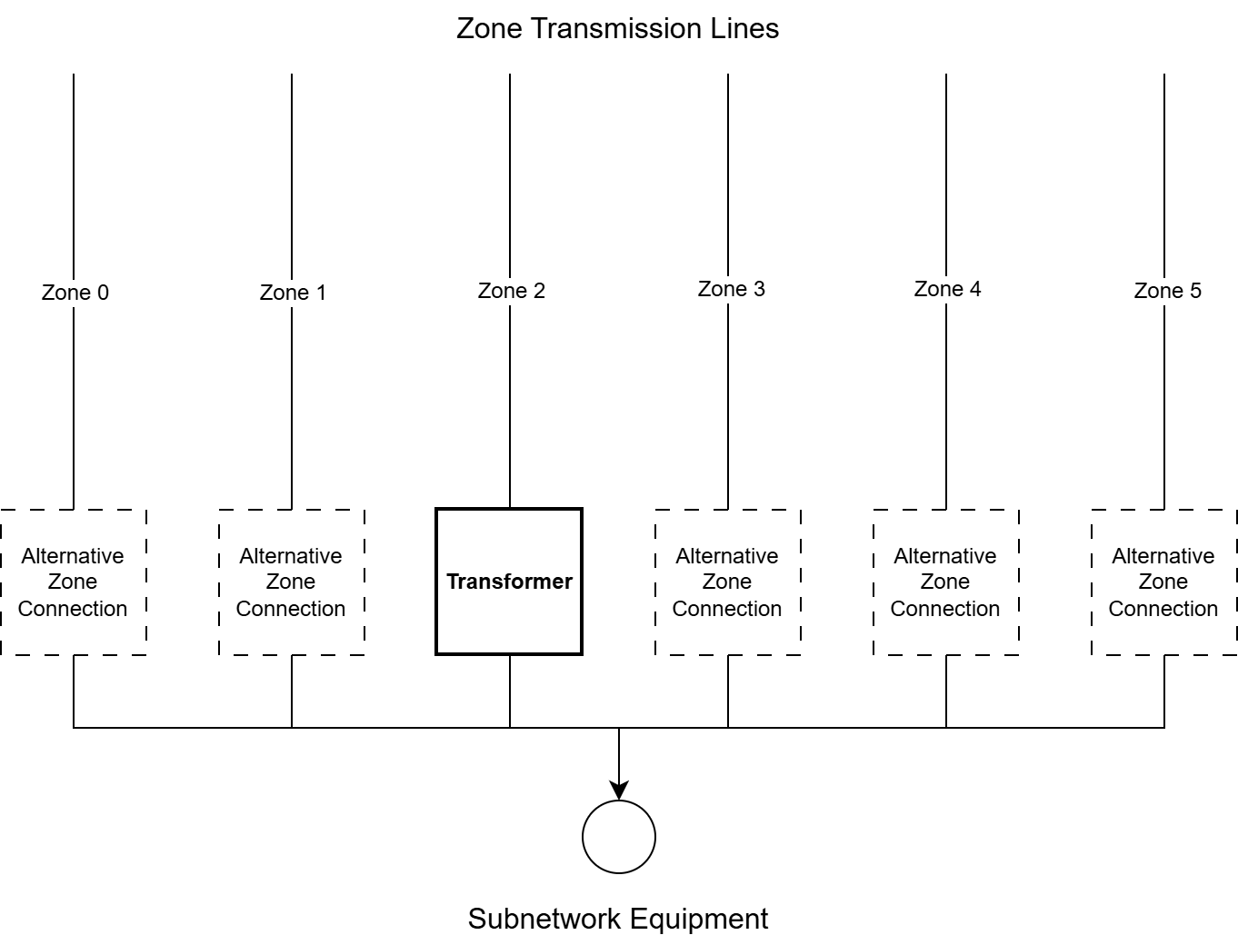
Changing a subnetwork’s zone assignment requires disconnecting the transformer from one zone cable and reconnecting to a different zone cable at the same location. The cable infrastructure remains unchanged; only the transformer’s connection point changes.
When to Reassign Subnetworks
Subnetwork reassignment makes sense when:
Priority classification changes: Equipment that was non-critical becomes critical (or vice versa). Reassigning to appropriate priority zones ensures correct load shedding behavior.
Zone capacity limits approached: A zone’s requested potential nears its transformer capacity. Shifting subnetworks to the next priority zone creates headroom.
Reassignment does not address:
Cross-region requirements: Multi-zone access only operates within regions. Moving subnetworks between regions requires new transmission and distribution cabling.
Insufficient regional capacity: If total regional requested potential exceeds generation capacity, reassigning subnetworks between zones does not solve the underlying shortage. Add generation capacity or create new regions instead.
Monitoring Grid Stability
Power regulation depends on measuring grid performance to detect degradation before failures occur. Monitoring tracks budget adequacy and actual consumption to trigger alerts when the grid approaches critical limits.
Budget ratio: Calculated budget divided by requested usage. This metric reveals whether generation capacity adequately supports usage demands. Values greater than 1 indicate adequate generation capacity with headroom for growth. Values at or below 1 indicate energy shortfall—generation cannot sustain requested loads, triggering load shedding.
Actual regional consumption: This metric tracks actual power consumption independent of what subnetworks request. Sustained high consumption approaching cable capacity limits (as discussed in Cable Capacity and Risk Assessment) signals the need for infrastructure upgrades or regional expansion. For measurement calculation see Appendix A3. Monitoring Cable Capacity.
Future Considerations
Some equipment operates intermittently with high power draw—fuel production, advanced fabrication, or recycling. These batch loads create scheduling challenges: running them within generalized regions may require increased generation infrastructure, that would in most cases be underutilized.
Overflow regions provide dedicated capacity for opportunistic batch loads that run only when surplus exists beyond base facility requirements. During periods of excess generation (solar and wind storms), overflow regions receive power for low-priority, deferrable systems. And during constrained periods, overflow regions would receive zero allocation, separating batch scheduling from base facility load management.
Links to Implementation
For operators ready to implement this Microgrid Architecture within their own base, the following implementation guide walks through the full construction process—complete with layout considerations, materials, and programmable logic:
Power II: Scaling Beyond Centralized Infrastructure - Implementation guide covering IC10 code, physical layout, component specifications, and deployment procedures for multi-regional power distribution across facility locations.
Appendix
A1. Capacity Utilization Tracking
Equipment rarely consumes its full rated capacity continuously. A 135 W filtration might draw 10 W when idle or an 800 W turbo volume pump might draw 675 W during active processing. Requested potential (the cumulative maximum that power equipment could draw) differs from actual consumption (what equipment currently draws).
This gap between potential and actual creates allocation challenges. If the system allocates based on requested potential alone, it overestimates power requirements and unnecessarily restricts loads. If it allocates based on instantaneous actual consumption, the load balancer cannot reliably determine when to restore previously shed loads—a system drawing low power might need to absorb the restored load.
Exponential moving average (EMA) tracks the relationship between actual consumption and requested power over time, providing stable capacity utilization estimates despite short-term fluctuations.
The capacity utilization factor represents:
Tracked over time with EMA:
Where:
τ (time constant): 1.5 × generation cycle period
Δt (tick interval): Controller update frequency (typically 0.5 seconds)
α (learning rate): Δt / τ
For solar power with a 20-minute day/night cycle:
This time constant captures behavior over 1.5 full cycles, smoothing transient spikes while tracking genuine load pattern changes. The system converges to stable estimates within 3-5 cycles.
A2. Power Budget Calculation
Available power derives from battery state and expected offline duration:
Where:
charge: Current stored energy (joules or watt-seconds)
offline_period: Expected duration without generation (seconds)
cap_util_ema: Current capacity utilization estimate
The offline period varies by generation source:
Solar panels: 600 seconds (nighttime duration)
Wind turbines: Varies with weather patterns
Coal generators: Fuel resupply interval
Mixed generation: Shortest expected gap between any generation source
Dividing by cap_util_ema translates from actual watts (that the battery can sustain) to potential watts (what zones request). If systems typically consume 20% of their requested potential (cap_util_ema = 0.2), then 1000 W of actual battery budget supports 5000 W of requested potential.
A3. Monitoring Cable Capacity
Monitoring cable capacity requires tracking actual power consumption at the regional level using exponential moving average with the same parameters discussed in Appendix A1. Capacity Utilization Tracking:
A4. Glossary
This glossary defines the terminology specific to the Microgrid Architecture documented in this article. For broader Stationeering Systems terminology, refer to the Terminology Reference.
Budget Ratio — Calculated power budget divided by requested usage. Values greater than 1 indicate adequate generation capacity; values at or below 1 indicate energy shortfall requiring load shedding.
Distribution Line — Cables connecting subnetwork connection points to equipment groups.
Dual-Region Interconnection — Equipment (typically doors and airlocks) that connects to both regions simultaneously, drawing power from whichever region is operational.
Independent Systems — Systems that exist within regions without cross-regional coordination or failover. Accepts complete downtime if their region fails.
Load Shedding — Controlled disconnection of lower-priority subnetworks when available power budget becomes insufficient to support all requested loads.
Multi-Zone Access — Infrastructure design where all zone transmission lines route to every subnetwork location, enabling zone reassignment by moving transformer connections without cable rework.
N+1 Redundancy — Load distribution across N+1 regions where N regions provide 100% of required capacity during normal operation. Can tolerate a single-region failure without service interruption.
Overflow Region — Dedicated capacity for opportunistic batch loads that run only when surplus power exists beyond base facility requirements. Receives zero allocation during constrained periods.
Passive Battery Backup — Manual-activation battery system that provides additional power protection. Charges from regional power but requires manual activation, preserving battery during compound failures.
Requested Potential — The cumulative maximum power that equipment could draw under peak operation. Used for capacity planning and allocation decisions.
Transmission Line — Heavy or super heavy cables delivering power from the battery array to regional and zonal distribution points. Provides the infrastructure sized for regional capacity.
Uncharacterized Loads — Infrastructure power consumption that doesn’t route through zone-managed subnetworks: transformer base power, controller operation, battery charging for backup systems, and generation management equipment.
Content developed in collaboration with Anthropic’s Claude, used for technical documentation structure, engineering analysis, and editorial refinement.